A little bit of GDAL/OGR appreciation
If there had to be one single tool to work with spatial data, I think GDAL/OGR would be the first name to come to mind. Its usages range from raster to vector, it can be used as command line, imported as a library in many languages through bindings developed by the community, many applications provide UI to parameterize and run GDAL etc. Its versatility makes it an amazing tool to work with spatial data in a lot of different contexts, but it’s sometimes underestimated or even misunderstood.
We will quickly introduce GDAL/OGR, then give some examples of usage to help for some quick starts.
What is GDAL/OGR?
GDAL/OGR (Geospatial Data Abstraction Library/OpenGIS Simple Features Reference Implementation) is a library for working with raster and vector geospatial data formats, coded mainly in C++, C and Python. The first release dates from 2000, and the project has now more than 450 contributors at the time of writing. This is a very active project with regular releases.
The project is composed of two parts: the raster processing library GDAL and the feature processing library OGR, both merged during the release of GDAL 2.0. When working with raster data you will use programs prefixed with gdal (gdal_translate, gdalwarp etc.) while vector data will use ogr prefixed scripts (ogrinfo, ogr2ogr etc.). When talking aboutt GDAL, both libraries are included, and we’ll do the same from here.
As its name suggests, GDAL abstracts data in order to standardize its way of interacting with it. The driver creates the interface between the data source and the tools, allowing to focus on the logic of the process rather than how to read or write the data. This makes it a very extensible project; including a new format of data source requires to write a new driver, nothing more. You could see that the list of supported formats is quite something, either raster or vector.
GDAL describes itself as a translator, meaning that data come from a source and goes to its destination. Translations can occur at different moment during the process, during reading or by the script called. These translations can occur on multiple axis as well, we could for example:
- Extract a subset of source data depending on a region of interest.
- Extract a subset of source data based on an attribute.
- Reproject data into a different coordinate system.
- Merge a series of data files into a single one.
- etc.
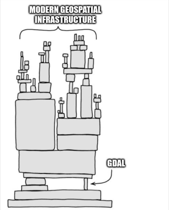 Source unknown, if it’s your image and you want to be cited please leave a comment
As an open source project with a permissive MIT license, GDAL is used by many projects, open source or proprietary, to process geospatial data. If you’ve used QGIS, ArcGIS, FME or PostGIS, you’ve used GDAL under the hood.
Why would I use it?
Weirdly, even though GDAL is basically everywhere there is geospatial data to be moved, it’s not so much acknowledged by GIS people, or at least it’s not really used on its own. If you read this, you definitely use GDAL, but maybe without noticing.
Ok but why would I complicate my life with some command lines when the same tool is being used by a software that provides me a user interface easier to use?
While it’s much intuitive to explore geospatial data through a user interface such as QGIS, where you can interactively load your data, chose the process you want to apply, its parameters, and visualize the results, things get a bit more complicated once you’ve done the exploratory part and want to reapply your newly defined process to new data. Repeating operations becomes quickly tedious and error-prone. You could use a tool such as the Model Designer from QGIS (amazing little tool, check it if you repeat a lot of operations in QGIS), but how do you schedule your process to be started when you’re not able to launch it manually?
If you use a heavy client ETL such as FME, try once to compare the difference in speed between a simple table transfer done by launching a FME workspace (using a command line) and a simple ogr2ogr command, there is at least an order of magnitude of difference.
It’s about using a tool designed for a purpose as efficiently as possible.
How to install?
We’ll assume you have no installation of GDAL yet, but just to make sure you can try:
1
gdalinfo --version
which gives:
1
GDAL 3.4.1, released 2021/12/27
If it’s not installed you can refer to the installation instructions from GDAL website.
For example, I’m working on Ubuntu 22.04, for which the GDAL package is the 3.4.1. The latest version can be installed by downloading the latest release, but I usually stick with the provided version for my platform, unless I need a specific update.
1
2
apt update
apt install gdal-bin
And you should be good!
You might already have GDAL installed through another software like QGIS, be careful during the installation, multiple installations might interfere and create warnings or errors. On Windows you can use the OSGeo Shell to access any tool from the OSGeo ecosystem.
And how do we use it?
It’s easy, you just need to be comfortable with command lines. If you’ve mostly worked with user interfaces it might look scary, but it really is not complicated.
Access metadata
The first thing we usually do with data is to have some information about it. Let’s try to see the metadata of a random .jpeg:
1
gdalinfo gdal.jpeg
1
2
3
4
5
6
7
8
9
10
11
12
13
14
15
16
17
18
19
20
21
22
23
24
25
26
27
Driver: JPEG/JPEG JFIF
Files: gdal.jpeg
Size is 711, 882
Metadata:
  EXIF_Orientation=1
Image Structure Metadata:
  COMPRESSION=JPEG
  INTERLEAVE=PIXEL
  SOURCE_COLOR_SPACE=YCbCr
Corner Coordinates:
Upper Left  (    0.0,    0.0)
Lower Left  (    0.0,  882.0)
Upper Right (  711.0,    0.0)
Lower Right (  711.0,  882.0)
Center      (  355.5,  441.0)
Band 1 Block=711x1 Type=Byte, ColorInterp=Red
  Overviews: 356x441, 178x221
  Image Structure Metadata:
    COMPRESSION=JPEG
Band 2 Block=711x1 Type=Byte, ColorInterp=Green
  Overviews: 356x441, 178x221
  Image Structure Metadata:
    COMPRESSION=JPEG
Band 3 Block=711x1 Type=Byte, ColorInterp=Blue
  Overviews: 356x441, 178x221
  Image Structure Metadata:
    COMPRESSION=JPEG
Easy right? And it’s not even georeferenced, it’s a .jpeg, a driver exists, it opens.
We can try the same with some vector data. We’ll have a look at what is going on in one of the PostgreSQL database hosted on my computer.
1
ogrinfo -ro PG:dbname=osm_suisse
1
2
3
4
5
6
7
INFO: Open of `PG:dbname=osm_suisse'
      using driver `PostgreSQL' successful.
1: planet_osm_line (Line String)
2: planet_osm_polygon
3: planet_osm_roads (Line String)
4: planet_osm_point (Point)
5: natural_polygons
And as we can see I have 5 layers in my database. Notice how we used the ogrinfo command for questioning vector data. Here ogrinfo (like gdalinfo) requires a dataset source as input, the syntax will depend on each driver, make sure to have a look at the documentation. For a PostgreSQL connection, the line could have looked like:
1
ogrinfo -ro PG:"dbname='osm_suisse' host='localhost' port='5432' user='x' password='y'"
We can extend the information that we want to see for each layer by adding the -al flag to the line. The option -so will summarize the output.
1
ogrinfo -ro -so -al PG:dbname=osm_suisse
1
2
3
4
5
6
7
8
9
10
11
12
13
14
15
16
17
18
19
20
21
22
23
24
25
26
27
28
29
30
31
32
33
34
35
36
37
38
39
40
41
42
43
44
45
46
47
48
49
50
51
52
53
54
55
56
57
58
INFO: Open of `PG:dbname=osm_suisse'
      using driver `PostgreSQL' successful.

Layer name: planet_osm_line
Geometry: Line String
Feature Count: 2137192
Extent: (626211.331305, 5706647.213604) - (1253686.695428, 6117386.570796)
Layer SRS WKT:
PROJCRS["WGS 84 / Pseudo-Mercator",
    BASEGEOGCRS["WGS 84",
        ENSEMBLE["World Geodetic System 1984 ensemble",
            MEMBER["World Geodetic System 1984 (Transit)"],
            MEMBER["World Geodetic System 1984 (G730)"],
            MEMBER["World Geodetic System 1984 (G873)"],
            MEMBER["World Geodetic System 1984 (G1150)"],
            MEMBER["World Geodetic System 1984 (G1674)"],
            MEMBER["World Geodetic System 1984 (G1762)"],
            MEMBER["World Geodetic System 1984 (G2139)"],
            ELLIPSOID["WGS 84",6378137,298.257223563,
                LENGTHUNIT["metre",1]],
            ENSEMBLEACCURACY[2.0]],
        PRIMEM["Greenwich",0,
            ANGLEUNIT["degree",0.0174532925199433]],
        ID["EPSG",4326]],
    CONVERSION["Popular Visualisation Pseudo-Mercator",
        METHOD["Popular Visualisation Pseudo Mercator",
            ID["EPSG",1024]],
        PARAMETER["Latitude of natural origin",0,
            ANGLEUNIT["degree",0.0174532925199433],
            ID["EPSG",8801]],
        PARAMETER["Longitude of natural origin",0,
            ANGLEUNIT["degree",0.0174532925199433],
            ID["EPSG",8802]],
        PARAMETER["False easting",0,
            LENGTHUNIT["metre",1],
            ID["EPSG",8806]],
        PARAMETER["False northing",0,
            LENGTHUNIT["metre",1],
            ID["EPSG",8807]]],
    CS[Cartesian,2],
        AXIS["easting (X)",east,
            ORDER[1],
            LENGTHUNIT["metre",1]],
        AXIS["northing (Y)",north,
            ORDER[2],
            LENGTHUNIT["metre",1]],
    USAGE[
        SCOPE["Web mapping and visualisation."],
        AREA["World between 85.06°S and 85.06°N."],
        BBOX[-85.06,-180,85.06,180]],
    ID["EPSG",3857]]
Data axis to CRS axis mapping: 1,2
Geometry Column = way
osm_id: Integer64 (0.0)
access: String (0.0)
addr:housename: String (0.0)
addr:housenumber: String (0.0)
[...]
And now we have the full detail of our layers; name, type, feature count, etc.
Basic translations
Now that we know what were working, with we can try to move some things around. Let’s start by exporting our vector data into a geopackage.
1
ogr2ogr -f GPKG exported_data.gpkg "PG:dbname=osm_suisse tables=planet_osm_point"
Here we’re exporting the table planet_osm_point into the exported_data.gpkg geopackage. The format can be recognized by the extension of the output file, but it’s safer to ensure the format by passing the argument -f. Again, each driver documentation will have its driver name to be used.
Add a filter
We can export a subset of our data, based on an attribute for example. Let’s say we want to export the points where the attribute addr:housenumber is not null, and we want to save it in another table in our newly created geopackage. We’d do something like:
1
ogr2ogr -update -f GPKG -where '"addr:housenumber" is not null' -nln only_housenumbers exported_data.gpkg "PG:dbname=osm_suisse tables=planet_osm_point"
We want to update our dataset (our geopackage) and not create a new one, so we use the -update option. The syntax of the -where parameter is a bit convoluted here since there is a special character in the column name, but with a simple name you’d just need a pair of quotes -where "housenumber" is not null".
Let’s have a look at our geopackage:
1
ogrinfo -ro -al -so exported_data.gpkg
1
2
3
4
5
6
7
8
9
10
11
12
13
14
15
16
17
18
19
20
21
22
23
24
25
26
27
28
29
30
31
INFO: Open of `exported_data.gpkg'
      using driver `GPKG' successful.

Layer name: planet_osm_point
Geometry: Point
Feature Count: 2146246
Extent: (626415.435591, 5736097.599850) - (1189428.532375, 6117386.570796)
Layer SRS WKT:
PROJCRS["WGS 84 / Pseudo-Mercator",
    BASEGEOGCRS["WGS 84",
        ENSEMBLE["World Geodetic System 1984 ensemble",
            MEMBER["World Geodetic System 1984 (Transit)"],
            MEMBER["World Geodetic System 1984 (G730)"],
            MEMBER["World Geodetic System 1984 (G873)"],
            MEMBER["World Geodetic System 1984 (G1150)"],
[...]

Layer name: only_housenumbers
Geometry: Point
Feature Count: 366561
Extent: (663719.309401, 5751784.044673) - (1167785.106794, 6072459.331387)
Layer SRS WKT:
PROJCRS["WGS 84 / Pseudo-Mercator",
    BASEGEOGCRS["WGS 84",
        ENSEMBLE["World Geodetic System 1984 ensemble",
            MEMBER["World Geodetic System 1984 (Transit)"],
            MEMBER["World Geodetic System 1984 (G730)"],
            MEMBER["World Geodetic System 1984 (G873)"],
            MEMBER["World Geodetic System 1984 (G1150)"],
            MEMBER["World Geodetic System 1984 (G1674)"],
[...]
The new layer has been added to the geopackage. Has the query been respected?
1
ogrinfo -ro -al -so -sql 'select * from only_housenumbers where "addr:housenumber" is null' exported_data.gpkg
1
2
3
4
5
6
7
8
9
INFO: Open of `exported_data.gpkg'
      using driver `GPKG' successful.

Layer name: SELECT
Geometry: Point
Feature Count: 0
Layer SRS WKT:
PROJCRS["WGS 84 / Pseudo-Mercator",
[...]
Yes! No data without addr:housenumber.
The
-sqloption is another way of filtering data, it allows you to pass a sql query in any of the sql flavor supported by the driver, you can even save your queries in a text file and pass the file to the-sqlparameter as-sql @path/to/my_file.
Geometric operations?
The -sql parameter can also be used to apply transformations to the data. We’ll request the same points, but this time we’ll create a buffer around them.
1
ogr2ogr -update -f GPKG -sql 'select ST_Buffer(way, 50) from planet_osm_point where "addr:housenumber" is not null' -nln buffered_only_housenumbers exported_data.gpkg "PG:dbname=osm_suisse tables=planet_osm_point"
And that’s it, we have our buffer around the points of interest. Here GDAL makes use of the internal capabilities of PostgreSQL and PostGIS by passing directly the request to the database, but the same command using the only_housenumbers layer from our geopackage would also be valid.
1
ogr2ogr -update -f GPKG -sql "select ST_Buffer(way, 50) from only_housenumbers" -nln buffered_only_housenumbers exported_data.gpkg exported_data.gpkg
In the case of PostgreSQL/PostGIS you can write the
-sqlparameter like you would write your queries directly into the database. They are passed directly to the database by GDAL.
This should give you a small idea of the things you can do with GDAL and how to start experimenting.
Final words
Well that was a lot more than expected. But GDAL really is a very strong and important tool. Diving into the details of all the available options, both for the command AND the drivers, is not a small task, but understanding how to navigate around and find the information that you need to process your data as you wish can go a long way. Manual and repeated tasks can be replaced to help to focus on more pertinent work, process time can be (by experience) reduced drastically depending on the tools you’re initially using. And if you’re working on data hosted on a server without graphic interface, well you have a tool to get the info you need!
Obviously GDAL alone can’t do everything and has its imperfections; I’ve really struggled with installations in the past (Python binding might have bested me at some point), and the number of parameters is a bit overwhelming. But once you have it working it does the job, and really well.
If you can, use GDAL.